
Tuning kNN and Opacity Pruning in 3DGS Simplification
A field guide to the seven parameters that control 3DGS simplification: ratio, kNN, merge cap, opacity prune, SH degree, and SOR outlier filtering.
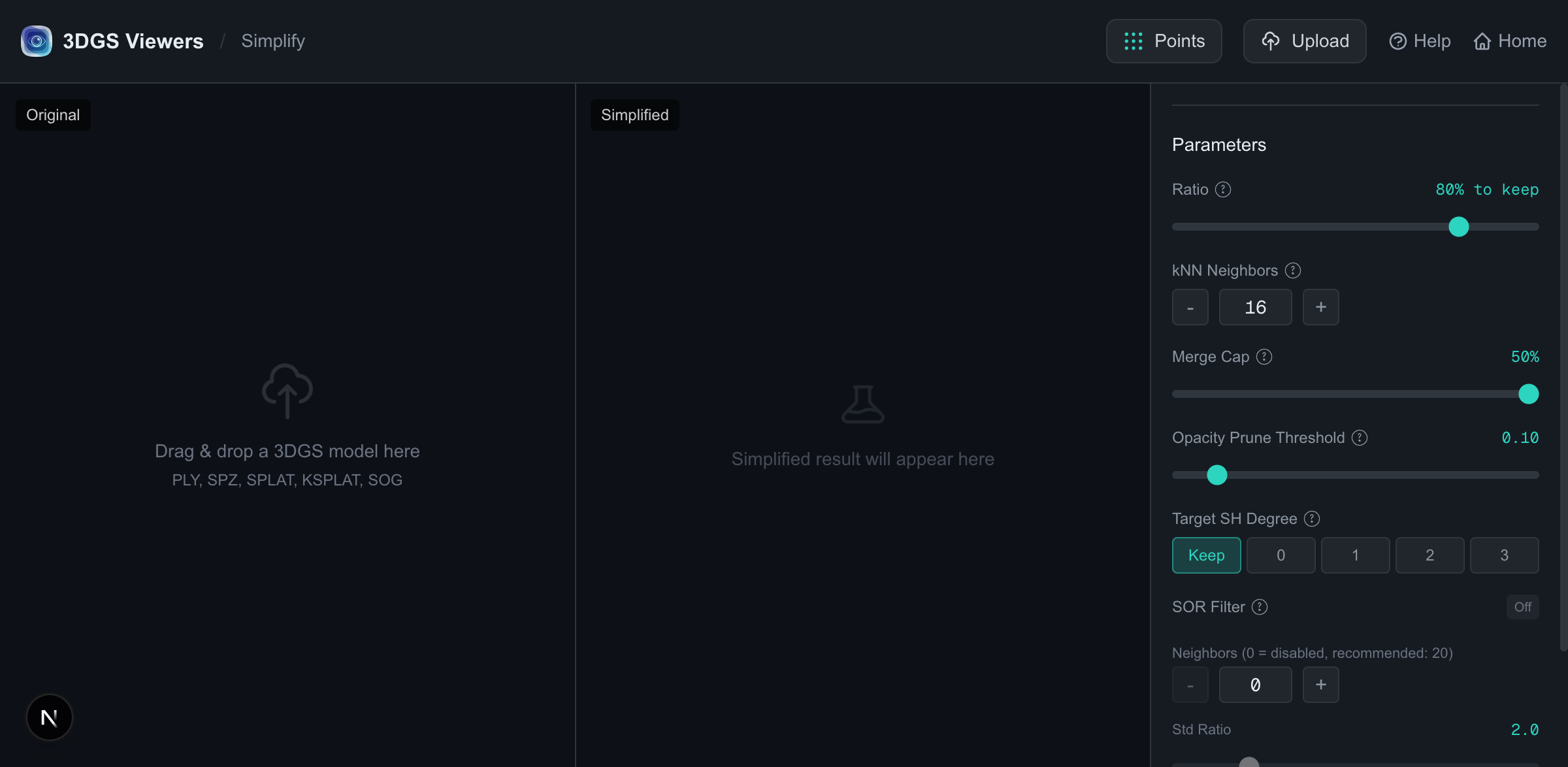
The 3DGS Simplify tool exposes seven parameters. If you have only ever moved the Ratio slider, you are leaving a lot of quality and file size on the table. Each parameter attacks a different kind of waste in a trained model, and most of them compose. This is a field guide to all seven: what each does, when to reach for it, and the trade-offs.
If you want the workflow-level overview first, read the compression article. This piece assumes you know the basic flow and want to tune.
1. Ratio — the master lever
Range: 0.01–1.0 (a keep ratio, not a removal ratio). Default 0.8.
This is how many of the original Gaussians survive after kNN merging. Everything else gets absorbed into neighbors. 80% is a safe default; below ~50% you start trading visible quality, and the exact cliff depends entirely on the scene. There is no universal “right” number — always verify with SSIM on the views that matter.
One detail that catches people: the ratio is approximate. The kNN merge process is guided by the ratio and the merge cap together, so the final splat count will be close to but not exactly original × ratio. Check the reported splats-reduction number in the result panel.
2. kNN Neighbors — how wide the merger looks
Range:1–64. Default 16.
When a Gaussian is removed, its visual contribution is distributed across its nearest neighbors. kNN Neighbors sets how many neighbors participate in that merge (using moment matching to preserve position, scale, rotation, and color statistics).
- Low k (e.g. 4–8): each removed splat is absorbed by very few neighbors. Faster, but merges are more local and can leave visible lumps on dense regions.
- Default (16): a good general-purpose balance.
- High k (32–64): merges spread further, producing smoother results on smooth surfaces but potentially blurring thin detail. Slower because the neighbor search is the expensive step.
If your simplified model looks “lumpy” on what should be a smooth surface, raise k. If fine detail (hair, foliage, text) is being smeared, lower k.
3. Merge Cap — throttle each pass
Range:0.01–0.5. Default 0.5.
This caps what fraction of neighbors can be merged in a single pass. It is a stability control: a high cap lets the merger be aggressive per iteration (fewer passes, but more risk of overshooting), while a low cap makes each pass gentler (more stable, but you may need a slightly lower ratio to hit your target count). Unless you are seeing unstable results on a tricky scene, leave it at default.
4. Opacity Prune Threshold — kill the invisible tail
Range:0–1. Default 0.10.
Gaussians with opacity below this threshold are dropped outright, before merging. This is almost always free quality, because sub-0.10-opacity splats contribute almost nothing to the rendered image but still cost bytes and render time.
The tool shows a live opacity histogram under this control so you can see exactly what you would be removing. Read the histogram left to right: the leftmost bins are the nearly-transparent splats.
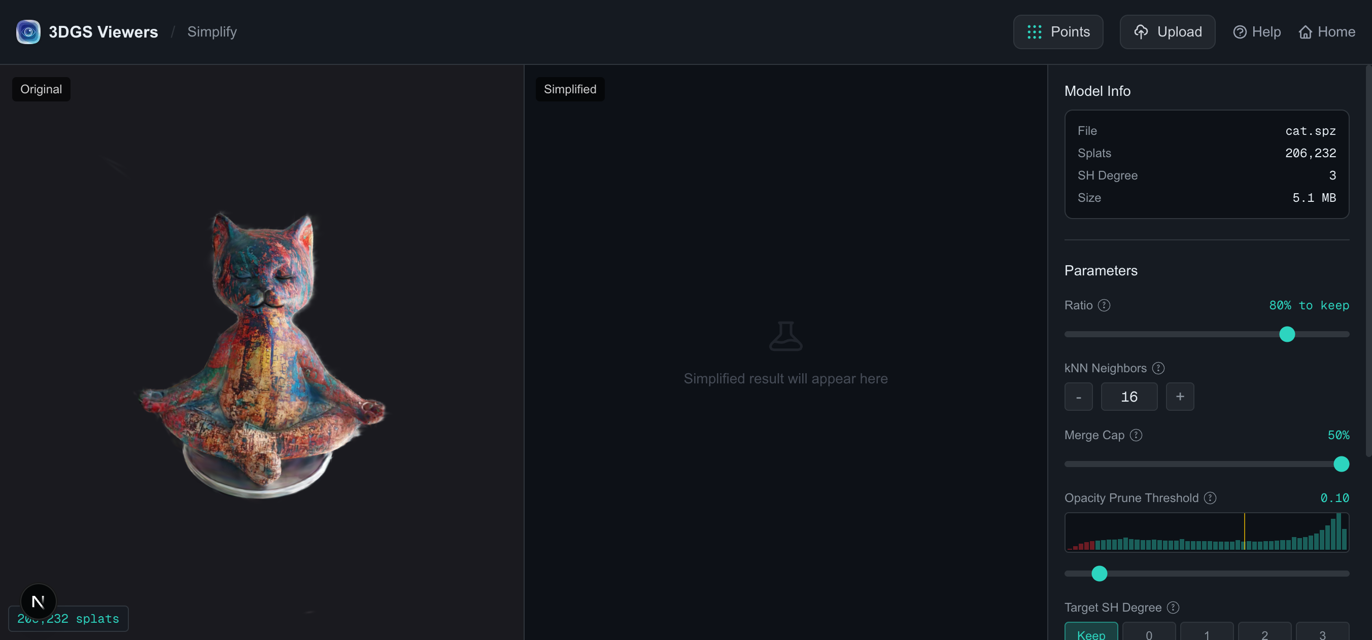
For the example model, the lowest bins hold thousands of splats each. Pushing the threshold from 0.10 to 0.15–0.20 removes a meaningful chunk of the model for free. Above ~0.30 you start cutting into visible detail — watch the SSIM number as you push.
5. Target SH Degree — trade view-dependent color for bytes
Options: Keep, 0, 1, 2, 3. Default Keep.
Spherical harmonics store view-dependent color — the way a surface shifts hue or specular highlight as you move around it. SH3 (the default for trained models) is the richest; each step down halves the SH data per splat at the cost of view-dependent fidelity.
| Setting | SH data per splat | What you lose |
|---|---|---|
| Keep | full SH3 | nothing |
| 2 | ~half | fine specular detail |
| 1 | ~quarter | most view-dependent color shifts |
| 0 | none (constant color) | all view-dependent effects; looks flatter |
For most web delivery, SH1 or SH2 is plenty. SH0 makes the model look noticeably flatter but is fine for matte surfaces (stone, fabric, concrete). Avoid SH0 for anything shiny or metallic — the loss is obvious.
6 & 7. SOR Filter — remove isolated outliers
Neighbors: 0–256 (0 = disabled). Std Ratio:0.1–10. Default Off.
Statistical Outlier Removal is a separate stage that removes Gaussians whose local density is statistically too low — in other words, isolated splats that are probably floaters or training noise. It is the right tool for the job described in removing floaters.
- Neighbors sets how many surrounding splats each candidate is compared against. 20 is a sensible starting point; higher is more robust but slower.
- Std Ratiois the sensitivity. A lower ratio is more aggressive (removes more). 2.0 is a standard default; drop to 1.0–1.5 for heavy cleanup.
SOR is opt-in because it is expensive on large models and because, unlike merging, it can remove legitimately sparse-but-real detail (e.g. isolated features on the edge of a scene). Turn it on only when you actually see floaters, and verify the result visually.
How the parameters combine
These are not mutually exclusive — they pipeline. A typical aggressive-but-safe web preset looks like:
| Stage | Parameter | Why |
|---|---|---|
| Remove invisible | Opacity prune = 0.15 | Free cleanup of the opacity tail |
| Merge | Ratio = 0.5, kNN = 16 | Halve the splat count with smooth merges |
| Trim color | SH degree = 1 | Drop most view-dependent data, keep bytes small |
| Cleanup (optional) | SOR neighbors = 20, ratio = 2.0 | Only if floaters remain |
Run that stack on a 200K-splat source and you typically land near 80–90K splats at SH1, which then converts to a small SPZ or SOG for delivery.
Opacity pruning happens before merging (correct — you do not want to spend merge effort on splats you are about to delete). SOR runs as its own stage. The tool handles the ordering for you; just be aware that the final splat count is a product of all the active stages, not just the ratio.
A tuning checklist
- Load the model, read the opacity histogram. Set Opacity pruneto the point where the left tail is exhausted (often 0.10–0.20).
- Set Ratio to your target (start at 0.7–0.8). Leave kNN at 16.
- Run. Calculate SSIM from your hero view.
- If SSIM is high (> 0.95) and you want smaller: lower the ratio, optionally drop SH degree to 2 or 1, re-run.
- If the surface looks lumpy, raise kNN. If fine detail is smeared, lower it.
- If you see isolated floaters after merging, enable SOR (neighbors 20, ratio 2.0) and re-run.
- Export to your delivery format.
Further reading
- Compressing Gaussian Splatting models — the workflow this tuning fits into.
- Removing floaters and outliers — when SOR is the right tool, in depth.
- Comparing 3DGS runs — how to read SSIM scores when tuning parameters.
- LightGaussian — the research on pruning and quantization that informs these defaults.
Try it in your browser
3DGS Viewer runs entirely in your browser — no installation, no upload required for the tools covered in this article. Pick a tool and start in seconds.